
Terrestrial laser scanning (TLS) can blanket a site with millions of returns per scan, but working at the scale of individual tree stems still means deliberate segmentation: separating ground from surface, finding stem bases in the ground cloud, then peeling branches away from trunks using geometry and density in lower dimensions. The same field campaign also supports a coarser question once bases are mapped: are those locations random, clustered, or uniform on the ground footprint?
Introduction
The high fidelity of LiDAR from TLS is attractive for detailed environmental modeling. Scanner sampling density can be tuned for nearly continuous coverage, and object shapes can be extremely well defined. As hardware and software improved, the bottleneck shifted from acquisition to processing: typical scans hold tens of millions of measurements, multi-scan objects are the norm, and workflows must be designed to finish in reasonable time. Often the first task is to classify and segment objects of interest from the bulk point cloud.
This project contributed a two-part workflow. Part one used alpha-disks on a ground cloud to propose tree-base regions, then buffers and GIS steps to clip candidate surface trees. Part two projected each candidate tree to the plane, built Voronoi-based density diagrams (scripts from the C177 toolbox by Daniel Radke), and used a global fifth-order polynomial surface in ArcGIS to outline high-density “stem cores” before clipping again in Maptek I-Site Studio.
Study system and data
Targets were main stems of blue-gum eucalyptus (Eucalyptus globulus) in the Grinnell Natural Area on the UC Berkeley campus. TLS was collected in May 2015 with a FARO Focus3D X130, with field support from Vishal Arya (then a UC Berkeley student): fifty moderate-resolution scans, target-based registration, and project-level accuracy reported at sub-centimeter agreement on control in FARO SCENE. That metric describes target agreement, not every canopy tip; upper canopy points are expected to be noisier where wind moves foliage between scans.
For interoperability, registered clouds were exported through vendor tools into indexed formats such as LAS and E57 (and LAZ where compression helped); LAStools and CloudCompare sat alongside ArcGIS and I-Site Studio in the practical toolchain.
TLS background
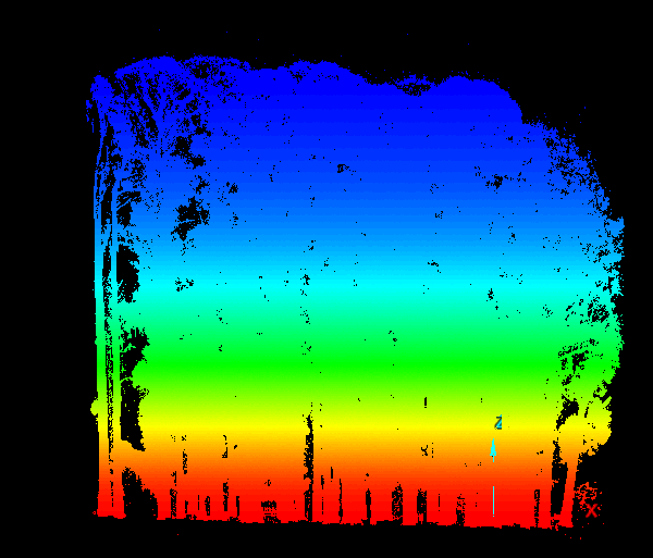
TLS systems measure range along each line of sight from azimuth and zenith; time-of-flight yields distance from the instrument to the reflecting surface. Under good conditions, ranges can be accurate to within a few millimeters. For visualization, returns are usually drawn as dimensionless points in X, Y, Z; the origin may sit at the scanner or at a reference scan when scans are registered together.
Ground versus surface in TLS
Ground points often exceed half of a single scan. Separating ground from surface is a common first segmentation step. Discrete-return scanners give one range per direction; full-waveform systems can yield multiple returns per pulse. For airborne LiDAR, “last return equals ground” is often defensible near nadir. For TLS, last returns frequently hit trunks, rocks, or buildings instead of bare earth, so a binning filter that keeps the lowest Z in each bin is usually safer than blind last-return filtering.
After classification, storing ground and surface in separate files speeds later processing and visualization.
Preprocessing
Beyond 2015 registration, ground points were extracted with a binning minimum-elevation filter; everything else was treated as surface. Both clouds were clipped to a bounding polygon that dropped temporary site clutter (topsoil piles, staged equipment). Finally, a minimum distance between points thinned the clouds (25 cm ground, 10 cm surface) to keep file sizes workable.
Part I: stem bases from the ground cloud
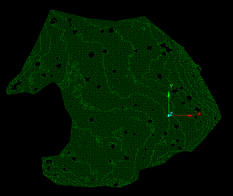
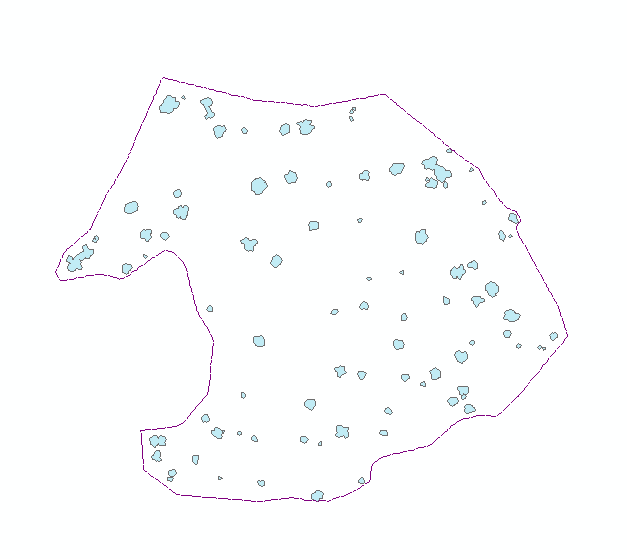
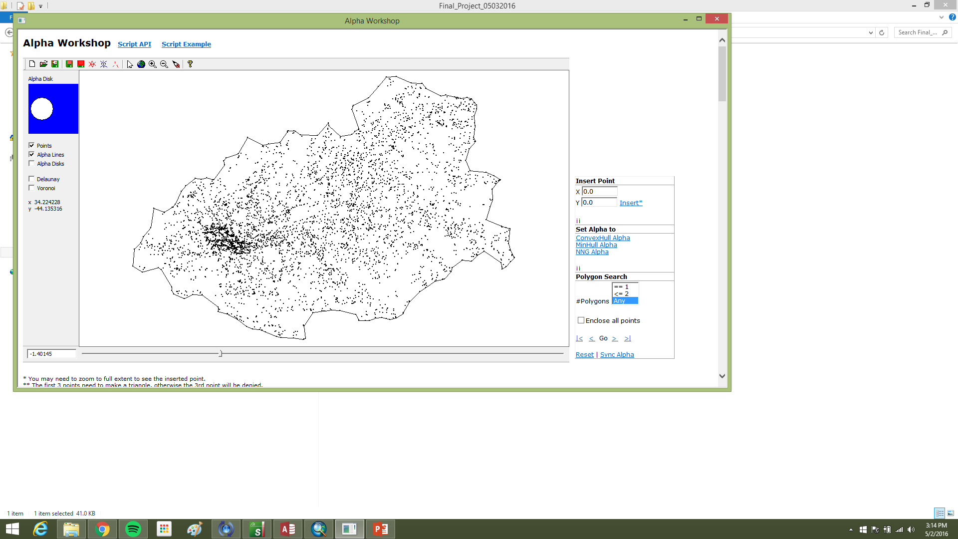
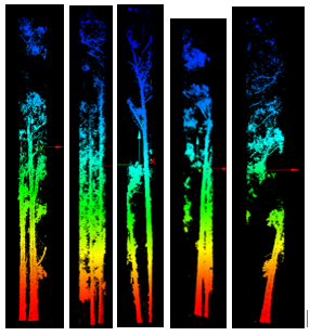
Even after thinning, the ground cloud was nearly continuous, with holes under stems where no ground returns exist. Those holes outline candidate tree bases at the data–no-data boundary. Nearest-neighbor graphs built with small-radius alpha disks (via the AEGIS tool distributed in C177) traced those internal boundaries more effectively than minimum-hull alpha shapes, which emphasize outer extents (Figure 2).
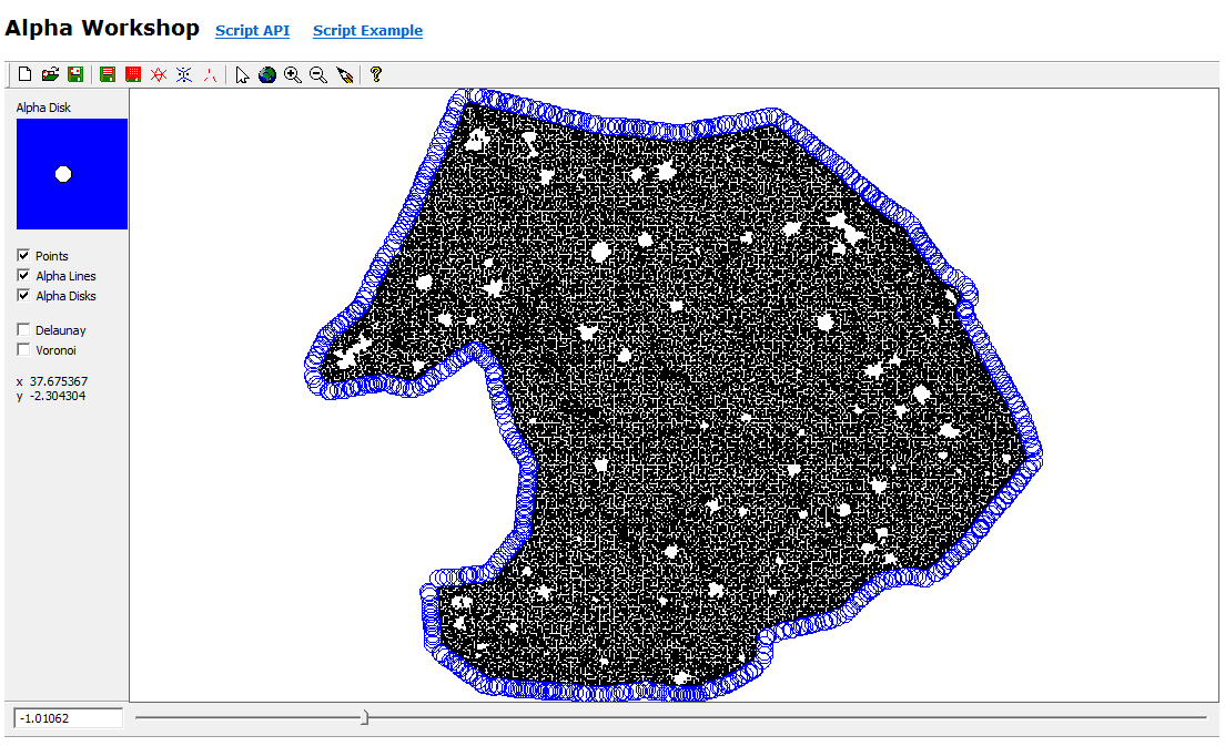
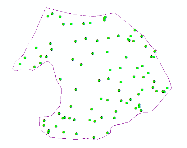
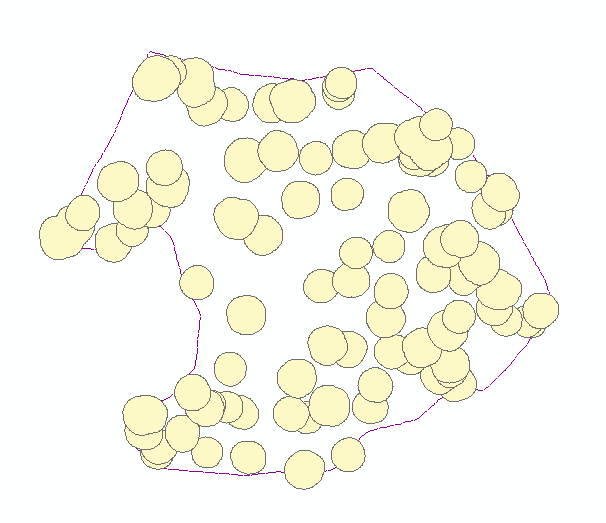
Alpha polylines exported to shapefiles were converted to polygons in ArcGIS (Feature to Polygon), dissolved where they overlapped or shared edges, and enriched with centroid coordinates. Those centroids became point features (Display XY Data). A two-meter buffer around each dissolved polygon was written to CAD, imported into I-Site Studio, and used with Filter by Polygon to pull surface points inside each footprint (Figure 3).
Each clipped cloud was rated good (single stem at the centroid), satisfactory (multiple stems but one wraps the centroid), or poor (no stem at ground). Part two focused on good cases.
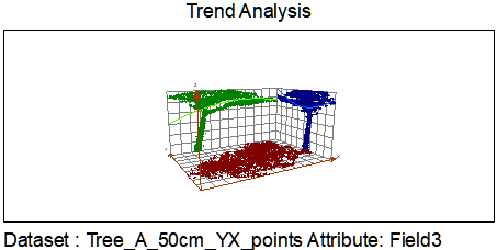
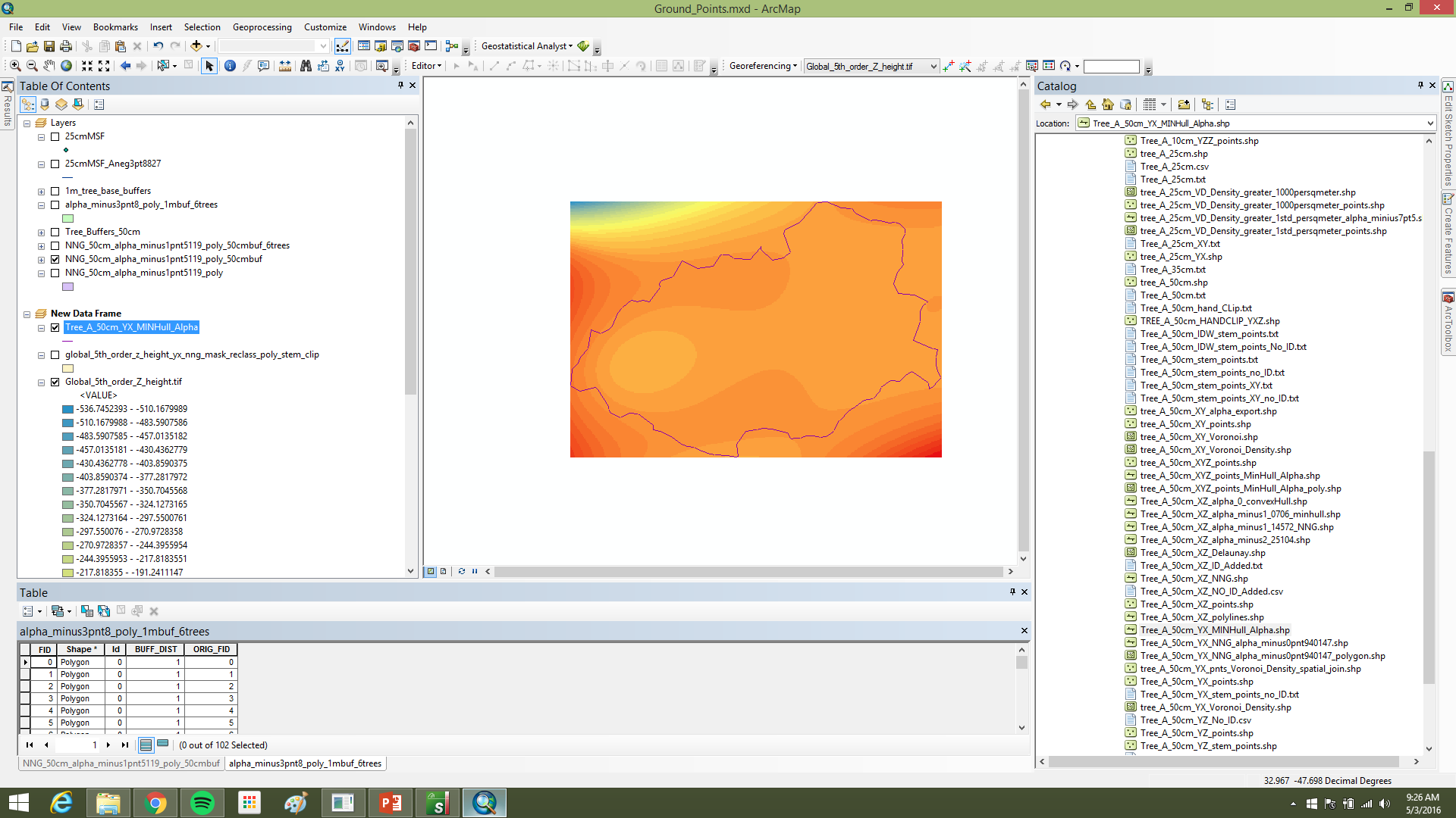
Part II: density on the plane and stem cores
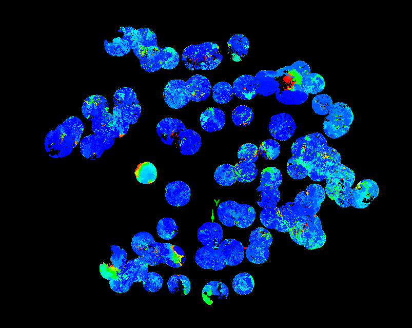
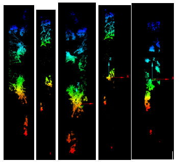
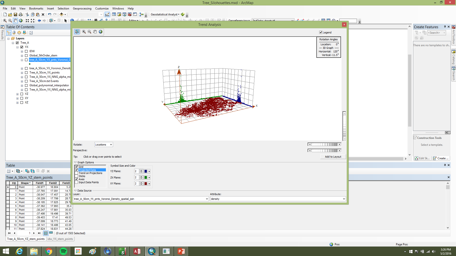
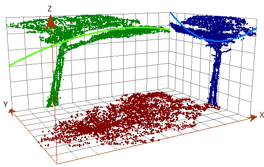
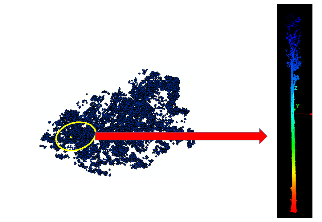
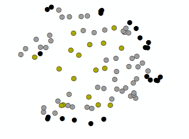
The working assumption was that, after projection to XY, the main stem occupies the densest part of the point field (Figure 4). Points were tessellated with Voronoi polygons; cell densities were joined back to points in ArcGIS using C177 toolbox code. A global fifth-order polynomial interpolated density across the 2D footprint; classification breaks isolated high-density cores. To reduce edge artifacts, the raster was clipped by a minimum-hull alpha shape from AEGIS before polygonization; polygons went to CAD for filtering in I-Site Studio (Figure 5).
Results
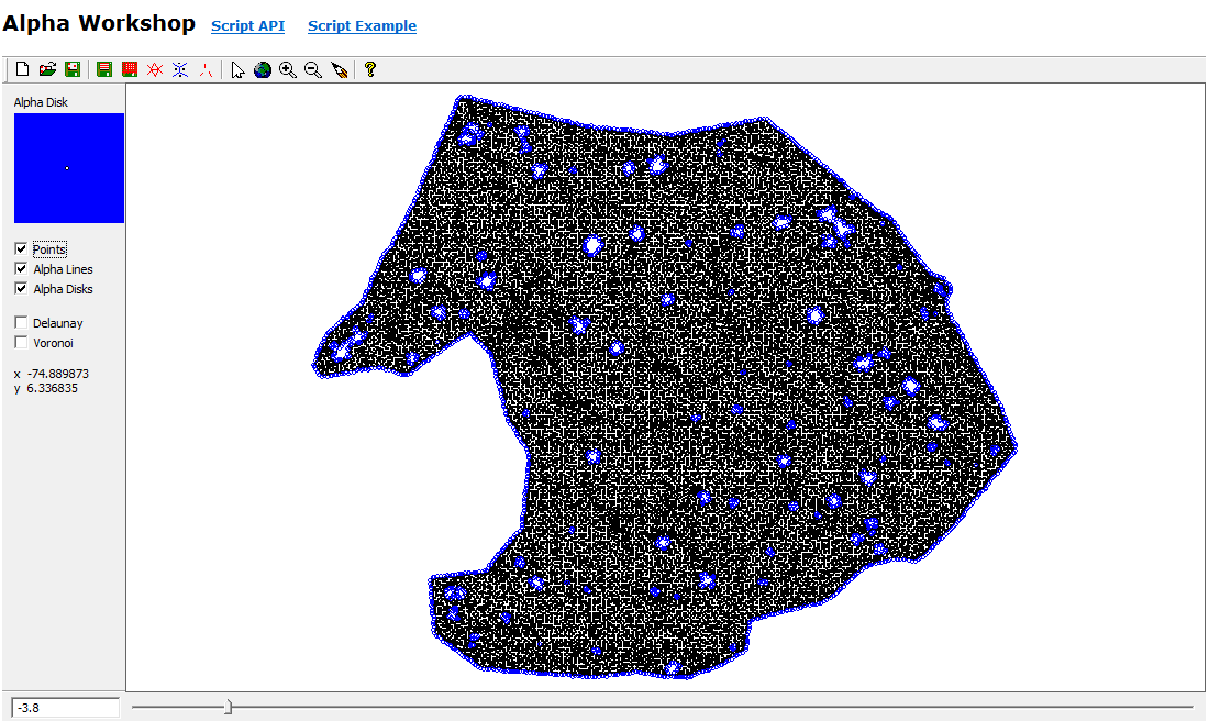
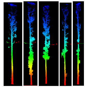
The NNG alpha (−3.8) was much smaller than the minimum-hull alpha (−1.1), which helped capture stem bases without bridging every non-target gap. One hundred twenty polygons came from line-to-polygon conversion; after dissolve, ninety candidates remained. Buffering into surface clouds yielded seventeen good, fifty satisfactory, and twenty-three poor extractions (Figure 6). Part two was only run on a handful of trees under time pressure, but Voronoi-attributed densities clearly peaked on stems (Figure 7), and the polynomial mask removed much of the branch wood while retaining the yellow high-density stem corridor in Figure 8.
Stem maps and point-pattern analysis (proposal thread)
The spring proposal used a slightly different emphasis: treat the workflow as building a stem map from the ground cloud first—alpha hull nearest-neighbor graphs (NNG), polygons, centroids as estimates of stem position or pith at the base—then hand those centroid points to geostatistics. Conceptually it read left to right: registered TLS → ground surface → stem footprints → centroid map → pattern summary. Stage I was registration and format normalization (FARO SCENE, I-Site Studio, LAStools). Stage II was ground filtering, NNG export, polygon and centroid construction in ArcGIS. Stage III was point-pattern analysis.
The null hypothesis was that centroid locations are spatially random across the grove footprint. Using ArcGIS toolboxes and R packages already available in the course stack, the intent was to reject H0 only if the pattern was significantly clustered or uniform at α = 0.05. That question complements Part I/II segmentation: even when individual buffers misbehave, Figure 9 is still a sample of where the ground cloud believed trees lived, which is the point pattern you would summarize at stand scale.
The written proposal included a conceptual diagram in the appendix tying the stages together; the quantitative segmentation narrative and figures in the sections above came from the later final submission.
Discussion and conclusions
The pipeline leans only on coordinates and densities already in a basic TLS deliverable, which keeps inputs simple and opens the door to scripting. Even partial automation on “satisfactory” cases could save manual classification time at stand scale. Buffer radii could be tuned: smaller where stems are tight and vertical, larger or elliptical where boles sweep.
Poor extractions clustered on the study-area edge (Figure 9), which suggests residual gaps in the ground cloud where off-plot trees were removed from the surface product but the ground hole remained. Checking original scans for deleted neighbors would test that explanation.
TLS workflows almost always need subsetting. The practical rhythm is subset for exploration, isolate features, then selectively merge points back when extra resolution is worth the cost. Segmentation is what makes massive clouds legible when projects scale beyond a single grove. Most of the intellectual work was never a single clever step but the sequencing: defensible ground filtering for TLS, thinning that respects oversampling, then geometry that respects how stems break the ground surface before density tricks on the plane.